Analysis of single-cell Hi-C data¶

Download of the fastq files
Demultiplexing
Mapping
Creation of Hi-C interaction matrices
Quality control
Removal of chromosomes / contigs / scaffolds
Normalization
Correction
Analysis
Bulk matrix

The analysis of single-cell Hi-C data deals is partially similar to regular Hi-C data analysis, the pre-processing of data i.e. mapping and the creation of a Hi-C interaction matrix and the correction of the data works can be adapted from a Hi-C data analysis. However, single-cell Hi-C deals with different issues as the be mentioned the pre-processing of the fastq files (demultiplexing) to associate the reads to one sample (to one cell). Everything that applies to Hi-C also applies to single-cell Hi-C expect in single-cell the work is done with a few thousand cells and not one. Additional, the read coverage in single-cell Hi-C is not in the hundreds of millions but on the used data form Nagano 2017 on average 1.5 million. This leads to other necessary treatments in the quality control of the samples and a need for a normalization to a equal read coverage for all cells.

In this tutorial we work with the ‘diploid’ data from Nagano 2017 (GSE94489).

Disclaimer

scHiCExplorer is a general tool to process and analysis single-cell Hi-C data. In this tutorial single-cell Hi-C data from Nagano 2017 (GSE94489) is used and scHiCExplorer provides a tool to demultiplex the FASTQ files. However, if all pre-processing (demultiplexing, trimming etc) is achieved by third-party tools and per cell the mapped forward and reverse strand files are present, scHiCExplorer can process them.

Disclaimer

The raw fastq data is around 1,04 TB of size and the download speed is limited to a few Mb/s by NCBI. To decrease the download time it is recommended to download the files in parallel if enough disk space is available. Furthermore, please consider the data needs to be demultiplexed and mapped which needs additional disk space.

If you do not want to download, demultiplex, map and build the matrices on your own, two precomputed raw scool matrices are provided on Zenodo in 1Mb and 10kb resolution. For this tutorial we use the 1Mb resolution of the matrix to reduce computation time. The 10kb takes significant longer and needs more memory to compute.

WARNING Please consider you need to convert the matrices first to the new scool file format as it is introduced with scHiCExplorer 5 and cooler 0.8.9. Use for this scHicManageScool and its update function.

Download of the fastq files ¶

As the very first step the raw, non-demultiplexed fastq files need to be downloaded. Please download the files directly from NCBI GEO and not e.g. from EMBL ENA, we have seen that these files miss the barcode information.

To download the fastq files the SRR sample number must be known, for not all samples only one SRR number was given, these samples were therefore not included in this tutorial.

SRR5229019  GSM2476401      Diploid_11
SRR5229021  GSM2476402      Diploid_12
SRR5229023  GSM2476403      Diploid_13
SRR5229025  GSM2476404      Diploid_15_16_17_18
SRR5229027  GSM2476405      Diploid_1_6
SRR5229029  GSM2476406      Diploid_19
SRR5229031  GSM2476407      Diploid_20
SRR5229033  GSM2476408      Diploid_2_14
SRR5229035  GSM2476409      Diploid_21
SRR5229037  GSM2476410      Diploid_22
SRR5229039  GSM2476411      Diploid_23
SRR5229041  GSM2476412      Diploid_24
SRR5229043  GSM2476413      Diploid_25
SRR5229045  GSM2476414      Diploid_26
SRR5229047  GSM2476415      Diploid_3
SRR5229049  GSM2476416      Diploid_4
SRR5229051  GSM2476417      Diploid_5_10
SRR5229053  GSM2476418      Diploid_7
SRR5229055  GSM2476419      Diploid_8
SRR5229057  GSM2476420      Diploid_9
SRR5507552  GSM2598387      Diploid_28_29
SRR5507553  GSM2598388      Diploid_30_31
SRR5507554  GSM2598389      Diploid_32_33
SRR5507555  GSM2598390      Diploid_34_35

Excluded: GSM2598386 / Diploid_27

Download the each file via:

$ fastq-dump --accession SRR5229019 --split-files --defline-seq \'@$sn[_$rn]/$ri\' --defline-qual \'+\'  --split-spot --stdout SRR5229019  > SRR5229019.fastq

Alternatively, download all with one command:

$ echo SRR5229019,SRR5229021,SRR5229023,SRR5229025,SRR5229027,SRR5229031,SRR5229033,SRR5229035,SRR5229037,SRR5229039,SRR5229041,SRR5229043,SRR5229045,SRR5229047,SRR5229049,SRR5229051,SRR5229053,SRR5229055,SRR5229057,SRR5507553,SRR5507554,SRR5507555 |  sed "s/,/\n/g" | xargs -n1 -P 22 -I {} sh -c "fastq-dump --accession {} --split-files --defline-seq \'@$sn[_$rn]/$ri\' --defline-qual \'+\'  --split-spot --stdout {}  > {}.fastq"

Please be aware that the additional parameters are only necessary if the files are downloaded via the bash. If you plan to download the files on hicexplorer.usegalaxy.eu and use there fastq-dump, the here shown additional parameters are handled in the background and only the accession number is required.

The downloaded fastq files must be in the following format:

@HWI-M02293:190:000000000-AHGUV:1:1101:12370:1000/1
NAAACTTCAAGGAAGCCAGAACAAGGATAGGAAAGNNNNGNNNNNNNNNNNNNNNNNNNNNNNNNNNNNNNTNNNNNNNNNNNNNNNNNNNNNNNNNNNNNNNNNNNNNNNNNNNNNNNNNNNNNNNNNNNNNNNNNNNNNNNNNNNNNNN
+
#8ACCGGGGGGGGGGFGGGGGGGGGGG9FFDFGGG####################################################################################################################
@HWI-M02293:190:000000000-AHGUV:1:1101:12370:1000/2
NNNNNNNN
+
########
@HWI-M02293:190:000000000-AHGUV:1:1101:12370:1000/3
NNNNNNNN
+
########
@HWI-M02293:190:000000000-AHGUV:1:1101:12370:1000/4
NNNNNNNNNNNNNNNNNNNNNNNNNNNNNNNNNNNNNNNNNNNNNNNNNNNNNNNNNNNNNNNNNNNNNNNNNNNNNNNNNNNNNNNNNNNNNNNNNNNNNNNNNNNNNNNNNNNNNNNNNNNNNNNNNNNNNNNNNNNNNNNNNNNNNNN
+
#######################################################################################################################################################
@HWI-M02293:190:000000000-AHGUV:1:1101:13757:1000/1
NCCCTGTACTGGGGCATATAAAGTTTTACATGCACNTNTTNNNNNNNNNNNNNNNNNNNNNNNNNNNNNNNANNNNNNNNNNNNNNNNNNNNNNNNNNNNNNNNNNNNNNNNNNNNNNNNNNNNNNNNNNNNNNNNNNNNNNNNNNNNNNN
+
#8BCCGGGGGFFFGGGGGGGGGGGGGGGGGGFGGG####################################################################################################################
@HWI-M02293:190:000000000-AHGUV:1:1101:13757:1000/2
NNNNNNNN
+
########
@HWI-M02293:190:000000000-AHGUV:1:1101:13757:1000/3
NNNNNNNN
+
########
@HWI-M02293:190:000000000-AHGUV:1:1101:13757:1000/4
NNNNNNNNNNNNNNNNNNNNNNNNNNNNNNNNNNNNNNNNNNNNNNNNNNNNNNNNNNNNNNNNNNNNNNNNNNNNNNNNNNNNNNNNNNNNNNNNNNNNNNNNNNNNNNNNNNNNNNNNNNNNNNNNNNNNNNNNNNNNNNNNNNNNNNN
+
#######################################################################################################################################################

Please check this before the demultiplexing starts. If this format is not present, the demultiplexing will not work and creates only an empty output folder.

Demultiplexing ¶

Each downloaded file needs to be demultiplexed. To do so the barcodes per sample and the SRR to sample mapping needs to be provided:

$ scHicDemultiplex -f "FASTQ_FILE" --srrToSampleFile samples.txt --barcodeFile GSE94489_README.txt --threads 20

scHicDemultiplex creates a folder ‘demultiplexed’ containing the demultiplexed fastq files split as forward and reverse reads and follows the scheme:

sample_id_barcode_RX.fastq.gz

For example:

Diploid_15_AGGCAGAA_CTCTCTAT_R1.fastq.gz

Please consider that the time to demultiplex the file SRR5229025, which itself is 4.1 GB takes already ~35 mins, to demultiplex the full 1 TB dataset will take around 6 days to compute.

Mapping ¶

After demultiplexing, each forward and reverse strand file needs to be mapped as usual in Hi-C as single-paired files. For this tutorial we use bwa mem and the mm10 index:

$ wget http://hgdownload-test.cse.ucsc.edu/goldenPath/mm10/bigZips/chromFa.tar.gz -O genome_mm10/chromFa.tar.gz
$ tar -xvzf genome_mm10/chromFa.tar.gz
$ cat genome_mm10/*.fa > genome_mm10/mm10.fa

$ bwa index -p bwa/mm10_index genome_mm10/mm10.fa

$ bwa mem -A 1 -B 4 -E 50 -L 0 -t 8 bwa/mm10_index Diploid_15_AGGCAGAA_CTCTCTAT_R1.fastq.gz | samtools view -Shb - > Diploid_15_AGGCAGAA_CTCTCTAT_R1.bam
$ ls demultiplexed |  xargs -n1 -P 5 -I {} sh -c "bwa mem -A 1 -B 4 -E 50 -L 0 -t 8 bwa/mm10_index demultiplexed/{} | samtools view -Shb - > {}.bam"

Creation of Hi-C interaction matrices ¶

As a last step, the matrices for each cell need to be created, we use the tool ‘hicBuildMatrix’ from HiCExplorer:

$ hicBuildMatrix -s  Diploid_15_AGGCAGAA_CTCTCTAT_R1.bam Diploid_15_AGGCAGAA_CTCTCTAT_R2.bam --binSize 1000000 --QCfolder  Diploid_15_AGGCAGAA_CTCTCTAT_QC -o Diploid_15_AGGCAGAA_CTCTCTAT.cool --threads 4

To make this step more automated, it is recommend to use either a platform like hicexplorer.usegalaxy.eu or to use a batch script:

$ ls *.bam |  tr '\n' ' ' | xargs -n 2 -P 1 -d ' ' | xargs -n1 -P1-I {} bash -c 'multinames=$1;outname=$(echo $multinames | cut -d" " -f 1 | sed -r "s?(^.*)_R[12]\..*?\\1?"); mkdir ${outname}_QC && hicBuildMatrix -s $multinames --binSize 1000000 --QCfolder  ${outname}_QC -o ${outname}.cool --threads 4' -- {}

After the Hi-C interaction matrices for each cell is created, the matrices are pooled together to one scool matrix:

$ scHicMergeToScool --matrices matrices/* --outFileName nagano2017_raw.scool

Call scHicInfo to get an information about the used scool file:

$ scHicInfo --matrix nagano2017_raw.scool

Filename: nagano2017_raw.scool
Contains 3882 single-cell matrices
The information stored via cooler.info of the first cell is:

bin-size 1000000
bin-type fixed
creation-date 2019-05-16T11:46:31.826214
format HDF5::Cooler
format-url https://github.com/mirnylab/cooler
format-version 3
generated-by cooler-0.8.3
genome-assembly unknown
metadata {}
nbins 2744
nchroms 35
nnz 55498
storage-mode symmetric-upper
sum 486056

Quality control ¶

Quality control is the crucial step in preprocessing of all HTS related data. For single-cell experiments the read coverage per sample needs to be on a minimal level, and all matrices needs to be not broken and contain all the same chromosomes. Especially the last two issues are likely to rise in single-cell Hi-C data because the read coverage is with around 1 million reads, in contrast to regular Hi-C with a few hundred million, quite low and therefore it is more likely that simply no data for small chromosomes is present. To guarantee these requirements the quality control works in three steps:

Only matrices which contain all listed chromosomes are accepted
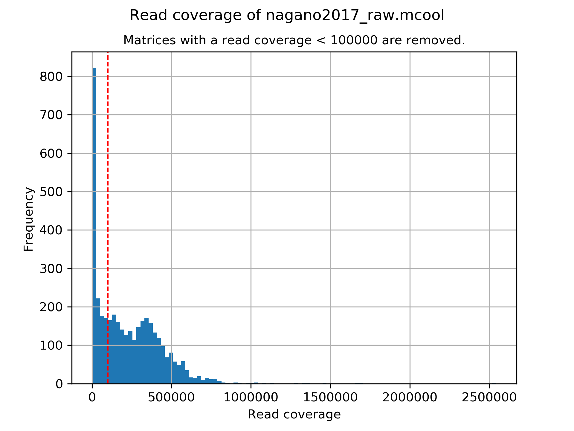
Only matrices which have a minimum read coverage are accepted
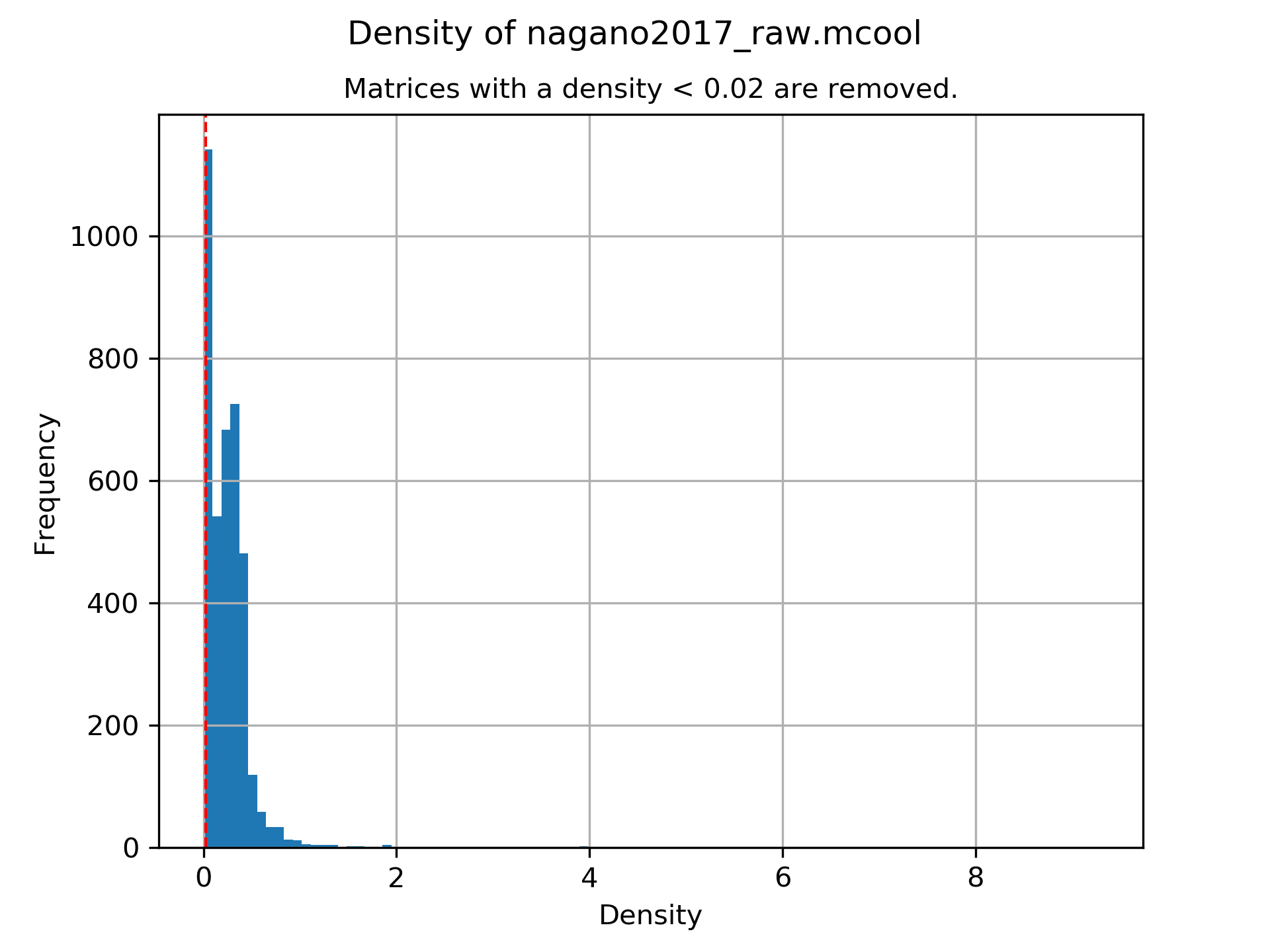
The matrix must have a minium density of recorded data points close to the main diagonal.

$ scHicQualityControl --matrix nagano2017_raw.scool --outputscool nagano2017_qc.scool --minimumReadCoverage 100000 --minimumDensity 0.02 --maximumRegionToConsider 30000000 --outFileNameReadCoverage read_coverage.png --outFileNameDensity density.png --threads 20 --chromosomes chr1 chr2 chr3 chr4 chr5 chr6 chr7 chr8 chr9 chr10 chr11 chr12 chr13 chr14 chr15 chr16 chr17 chr18 chr19 chrX

For this tutorial a minimum read coverage of 1 million and a density of 0.1% is used in range of 30MB around the main diagonal. The above command creates certain files:

A scool matrix containing only samples with matrices that passed the quality settings.
A plot showing the density of all samples. Use this plot to adjust the minimumDensity parameter.
A plot showing the read coverage of all samples, use this plot to adjust the minimum read coverage parameter.
A text report presenting quality control information.

# QC report for single-cell Hi-C data generated by scHiCExplorer 1
scHi-C sample contained 3882 cells:
Number of removed matrices containing bad chromosomes 0
Number of removed matrices due to low read coverage (< 100000): 1374
Number of removed matrices due to too many zero bins (< 0.02 density, within 30000000 relative genomic distance): 610
2508 samples passed the quality control. Please consider matrices with a low read coverage may be the matrices with a low density and overlap therefore.

These QC settings removes 2508 matrices:

$ scHicInfo --matrix nagano2017_qc.scool

Filename: nagano2017_raw.scool
Contains 3491 single-cell matrices
The information stored via cooler.info of the first cell is:

bin-size 1000000
bin-type fixed
creation-date 2019-05-16T11:46:31.826214
format HDF5::Cooler
format-url https://github.com/mirnylab/cooler
format-version 3
generated-by cooler-0.8.3
genome-assembly unknown
metadata {}
nbins 2744
nchroms 35
nnz 55498
storage-mode symmetric-upper
sum 486056

Removal of chromosomes / contigs / scaffolds ¶

A call of scHicInfo shows that in the first matrix 35 chromosomes are stored. Based on the problematic nature of the low read coverage it is quite likely that over the 3882 cells not all will have data present for all these chromosomes / contigs or scaffolds. It is now necessary to remove the contigs and scaffolds to achieve a good clustering results. The reason is, in clustering we operate directly on the matrices without the consideration of pixel to chromosome region relation. The assumption is that in cell 1 the i-th pixel is related to the same regions as in cell 1543. If some samples contain contigs and scaffolds, this cannot be guaranteed.

$ scHicAdjustMatrix -m nagano2017_qc.scool -o nagano2017_qc_adjusted.scool -t 20 --action keep --chromosomes chr1 chr2 chr3 chr4 chr5 chr6 chr7 chr8 chr9 chr10 chr11 chr12 chr13 chr14 chr15 chr16 chr17 chr18 chr19

Normalization ¶

Working with a few thousand samples makes it even more crucial to normalize the data to a similar read coverage level. scHiCExplorer normalizes to the lowest read coverage of all samples.

$ scHicNormalize -m nagano2017_qc_adjusted.scool -o nagano2017_normalized.scool --threads 20

Correction ¶

In Hi-C protocol the assumption is that each genomic local has the same sum of interactions. Usually this is not achieved and it is causing biases by over or under representing regions. To correct this we use the KR correction of matrices from Knight-Ruiz 2012.

$ scHicCorrectMatrices -m nagano2017_normalized.scool -o nagano2017_corrected.scool --threads 20

Analysis ¶

The analysis of single-cell Hi-C data investigates the chromatin folding changes during the cell cycle. To compute this, the clustering of the cells and a correct ordering within a cluster is the key step for this analysis.

scHiCExplorer uses a flatting approach to create out of the two dimensional 2D interaction matrices a one dimensional vector to have in the end a number of samples times number of bins^2 matrix. For example: Nagano 2017 has around 3000 cells and using a 1MB binning approach results for the mouse genome in 2600 times 2600 matrix. After flattening, the matrix which is used to operate on is 3000 * (2600 * 2600) = 3000 * 6760000.

Two approaches to apply clustering are possible:

Compute the clustering directly on the matrix.
Reduce the dimensions first and apply clustering.

Option one works if the resolution of the interaction matrices are not too high, i.e. 1MB leads to 6.7 million features which is already a lot, but todays computers can handle this. However, it looks different if the resolution is increased to e.g. regular Hi-C matrix resolution of 10kb. In this case the binned matrix is not 2600 * 2600, but 260000 * 260000 which is 67.6 billion. To work on such many features would be problematic in terms of computational time and, it is questionable if a computer with enough main memory is available. To overcome this, a dimension reduction is necessary. To reduce the number of dimensions scHiCExplorer provides three approaches: MinHash, SVL and Compartments.

The first approach uses a local sensitive hashing approach to compute the nearest neighbors, with it, it reduces the number of dimensions to the number of samples where each entry represents how close the samples are. Approach two, SVL for short vs long distances, computes per chromosome the ratio of the sum of short range contacts vs. the sum of long range contacts, the number of dimensions is therefore reduced to the number of to be considered chromosomes. Approach number three, compartments, computes the A/B compartments per chromosome and reduces the number of dimensions to the square root.

In Nagano 2017 a k-means approach is used to cluster the cells, however, the computed clusters with spectral clustering are of better quality.

Clustering on raw data ¶

The first approach clusters the data on the raw data using first, kmeans and second, spectral clustering. Warning: the runtime of kmeans is multiple hours (on a XEON E5-2630 v4 @ 2.20GHz with 10 cores / 20 threads, around 8 h).

$ scHicCluster -m nagano2017_corrected.scool --numberOfClusters 7 --clusterMethod kmeans -o clusters_raw_kmeans.txt --threads 20

$ scHicCluster -m nagano2017_corrected.scool --numberOfClusters 7 --clusterMethod spectral -o clusters_raw_spectral.txt --threads 20

The output of all cluster algorithms is a text file containing the internal sample name of the scool file and the associated cluster:

..code-block:: bash

/Diploid_3_CGTACTAG_GTAAGGAG_R1fastqgz 0 /Diploid_3_CGTACTAG_TATCCTCT_R1fastqgz 0 /Diploid_3_CTCTCTAC_AAGGAGTA_R1fastqgz 0 /Diploid_3_CTCTCTAC_ACTGCATA_R1fastqgz 0 /Diploid_3_CTCTCTAC_CGTCTAAT_R1fastqgz 0 /Diploid_3_CTCTCTAC_CTAAGCCT_R1fastqgz 0 /Diploid_3_CTCTCTAC_CTCTCTAT_R1fastqgz 0 /Diploid_3_CTCTCTAC_GTAAGGAG_R1fastqgz 0 /Diploid_3_CTCTCTAC_TATCCTCT_R1fastqgz 0 /Diploid_3_GCGTAGTA_AAGGCTAT_R1fastqgz 5 /Diploid_3_GCGTAGTA_CCTAGAGT_R1fastqgz 0 /Diploid_3_GCGTAGTA_CTATTAAG_R1fastqgz 0 /Diploid_3_GCGTAGTA_GAGCCTTA_R1fastqgz 0 /Diploid_3_GCGTAGTA_GCGTAAGA_R1fastqgz 0 /Diploid_3_GCGTAGTA_TCGACTAG_R1fastqgz 3 /Diploid_3_GCGTAGTA_TTATGCGA_R1fastqgz 4 /Diploid_3_GCTCATGA_AAGGAGTA_R1fastqgz 0 /Diploid_3_GCTCATGA_CGTCTAAT_R1fastqgz 0 /Diploid_3_GCTCATGA_CTAAGCCT_R1fastqgz 0 /Diploid_3_GCTCATGA_CTCTCTAT_R1fastqgz 0 /Diploid_3_GCTCATGA_GTAAGGAG_R1fastqgz 0

To visualize the results run:

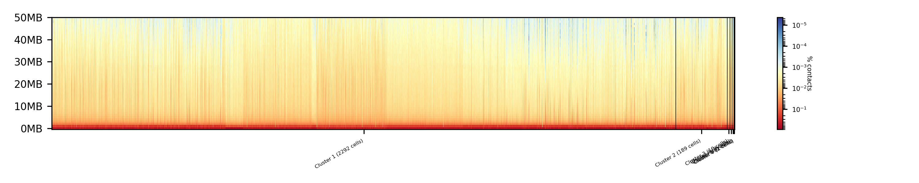
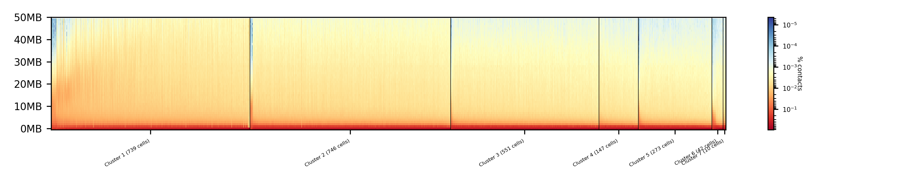
$ scHicPlotClusterProfiles -m nagano2017_corrected.scool --clusters clusters_raw_kmeans.txt -o clusters_raw_kmeans.png --dpi 300  --threads 20

The cluster internal ordering can be visualized in two ways: Either by the order the samples appear in the cluster output file or by sorting with the ratio of short vs. long range contacts. Default mode is the last one.

$ scHicPlotClusterProfiles -m nagano2017_corrected.scool --orderBy orderByFile --clusters clusters_raw_spectral.txt -o clusters_raw_spectral_order_by_file.png --dpi 300  --threads 20

$ scHicPlotClusterProfiles -m nagano2017_corrected.scool --orderBy svl --distanceShortRange 2000000 --distanceLongRange 12000000  --clusters clusters_raw_spectral.txt -o clusters_raw_spectral.png --dpi 300  --threads 20

../_images/clusters_raw_spectral_order_by_file.png

The profile of the clusters clearly shows that the algorithms fail to create a useful clustering of the samples and are not able to assoziate the cells to a cell cycle stage.

Clustering on kNN graph or PCA with exact methods ¶

To decrese the compute time, especially for kmeans, and to improve the clustering result the dimensions are reduced with two approaches: By computing a k-nearest neighbors graph and reduce the dimensions with it down to the number of samples or to compute the k-principal components of the matrix.

$ scHicCluster -m nagano2017_corrected.scool --numberOfClusters 7 --clusterMethod spectral -o clusters_knn_spectral.txt --threads 20 -drm knn

$ scHicPlotClusterProfiles -m nagano2017_corrected.scool --orderBy orderByFile --clusters clusters_knn_spectral.txt -o clusters_knn_spectral.png --dpi 300  --threads 20

$ scHicCluster -m nagano2017_corrected.scool --numberOfClusters 7 --clusterMethod kmeans -o clusters_knn_kmeans.txt --threads 20 -drm knn

$ scHicPlotClusterProfiles -m nagano2017_corrected.scool --orderBy orderByFile --clusters clusters_knn_kmeans.txt -o clusters_knn_kmeans.png --dpi 300  --threads 20

Comparing the two profiles of the clustering process, the dimension reduction with k-NN and kmeans works way better in assoziating samples to cell cycles. It can be clearly seen that cells with similar profiles are cluster together, however, not always this is the case. Considering cluster 6 shows on the right side 30 to 50 cells which profiles do not match the rest of the cluster. The spectral clustering shows, especially in comparison to spectral clustering without any dimension reduction no real improvement. Still the majorities of the cells are clustered to one cell cycle and the differentiation between the cell stages is not visible.

The PCA shows a different issue: Using a computer with 120 GB of memory is not enough to compute the PCA and is therefore not a method that is part of this analysis.

Clustering with dimensional reduction by local sensitive hashing ¶

Reducing the 2.6 million dimensions is a crucial step to improve the runtime and memory consumptions to acceptable level, especially if kmeans to cluster the single-cell Hi-C data is used. Under consideration of the clustering results on the raw data it is obvious that the dimensions are too high to get a meaningful clustering. scHiCExplorer uses the local sensituve hashing technique ‘minimal hash’ to reduce the number of dimensions to the number of samples, i.e. from 2.6 million to 3491. MinHash computes per samples for all non-zero feature id one hash value with one hash function and takes from all hash values the numerical minimum as the hash value for this hash function. With this approach a few hundred hash functions compute their minium hash value. In a next step the similarity between two samples is computed by counting the number of hash collisions, the more collisions two samples have, the more likely it is they share many non-zero feature ids.

$ scHicClusterMinHash -m nagano2017_corrected.scool --numberOfHashFunctions 1200  --numberOfClusters 7 --clusterMethod kmeans -o clusters_minhash_kmeans.txt --threads 20

$ scHicClusterMinHash -m nagano2017_corrected.scool --numberOfHashFunctions 1200 --numberOfClusters 7 --clusterMethod spectral -o clusters_minhash_spectral.txt --threads 20

To visualize the results run:

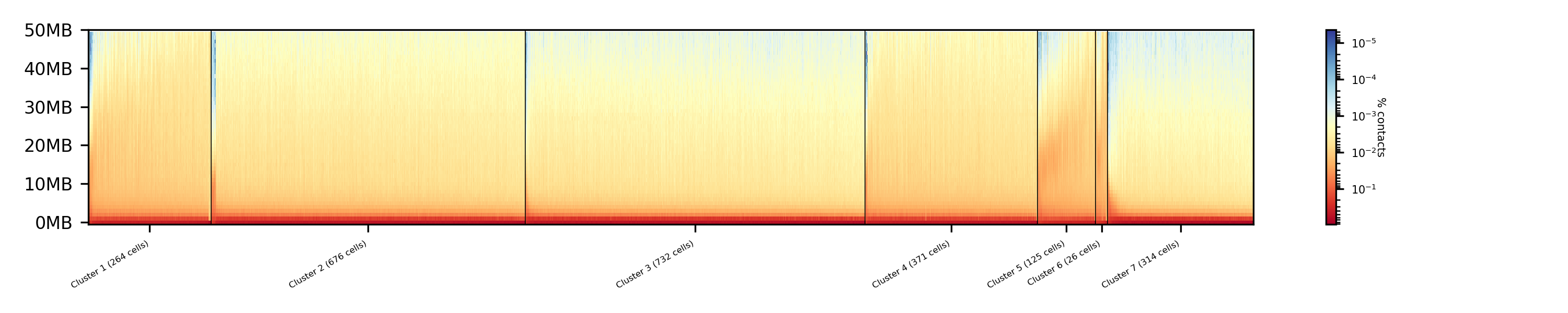
$ scHicPlotClusterProfiles -m nagano2017_corrected.scool --clusters clusters_minhash_kmeans.txt -o clusters_minhash_kmeans.png --dpi 300 --threads 20

$ scHicPlotClusterProfiles -m nagano2017_corrected.scool --clusters clusters_minhash_spectral.txt -o clusters_minhash_spectral.png --dpi 300 --threads 20

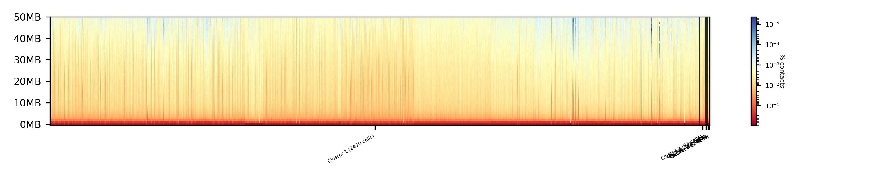
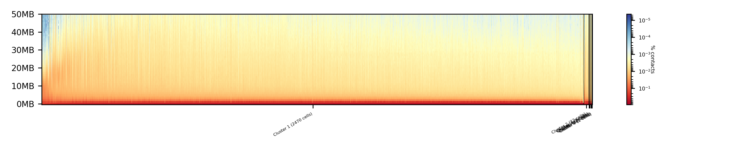
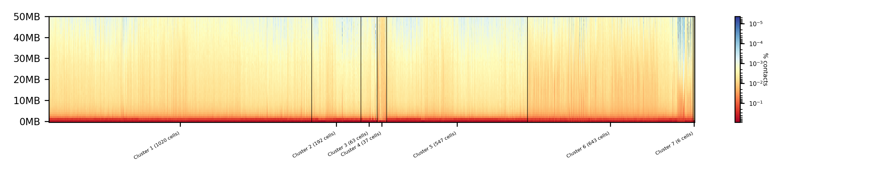
The clustered samples based on the dimension reduction with MinHash are way more meaningful in comparison to the raw clustered data:

../_images/clusters_minhash_spectral.png

The top image is clustered with kmeans, the bottom one with spectral clustering. Partially the results are quite equal e.g. in cluster 1 (kmeans) and 3 (spectral), however, the kmeans clustering seems to detect the fine differences in the chromatine structure better.

In comparison to the clustering based on raw data or the dimension reducted by exact kNN computation, the results with the approximate kNN based on MinHash seems to create better results.

Clustering with dimensional reduction by short range vs. long range contact ratios ¶

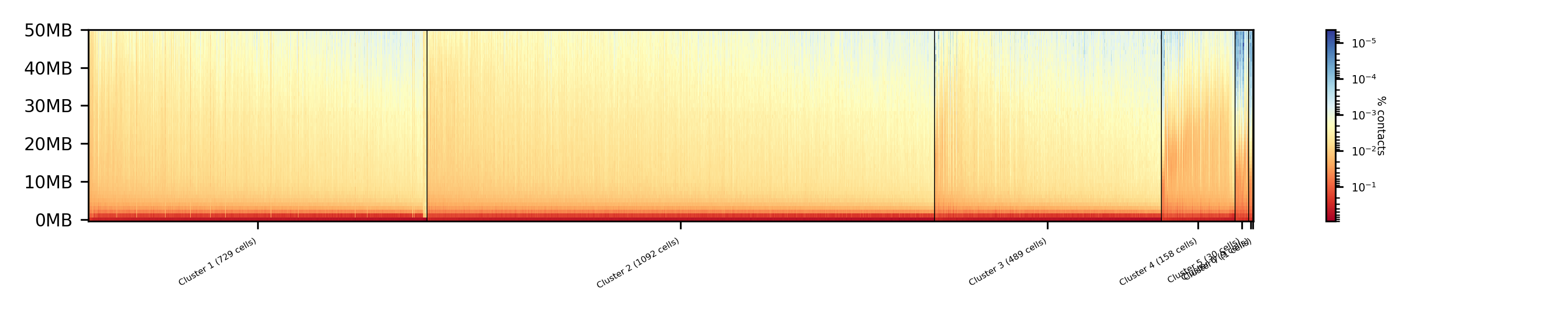
An important measurement to investigate the denisty of the folding structure of the chromatin is the ratio of the sum of short range and long range contacts. Nagano 2017 shows the ratio between genomical distance of less than 2MB and between 2MB to 12MB is the key region of contacts to be considered.

$ scHicClusterSVL -m nagano2017_corrected.scool --distanceShortRange 2000000 --distanceLongRange 12000000 --numberOfClusters 7 --clusterMethod kmeans -o clusters_svl_kmeans.txt --threads 20

$ scHicClusterSVL -m nagano2017_corrected.scool --distanceShortRange 2000000 --distanceLongRange 12000000 --numberOfClusters 7 --clusterMethod spectral -o clusters_svl_spectral.txt --threads 20

To visualize the results run:

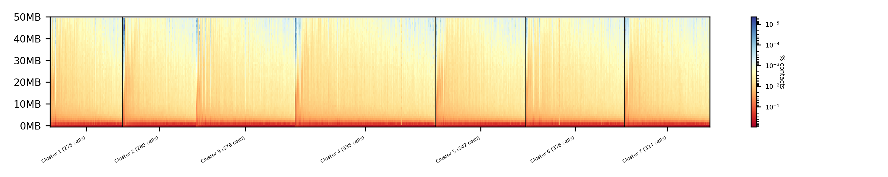
$ scHicPlotClusterProfiles -m nagano2017_corrected.scool --clusters clusters_svl_kmeans.txt -o clusters_svl_kmeans.png --dpi 300 --threads 20

$ scHicPlotClusterProfiles -m nagano2017_corrected.scool --clusters clusters_svl_spectral.txt -o clusters_svl_spectral.png --dpi 300 --threads 20

The results of the clustering with the SVL dimension reduction technique:

Clustering with dimensional reduction by A/B compartments ¶

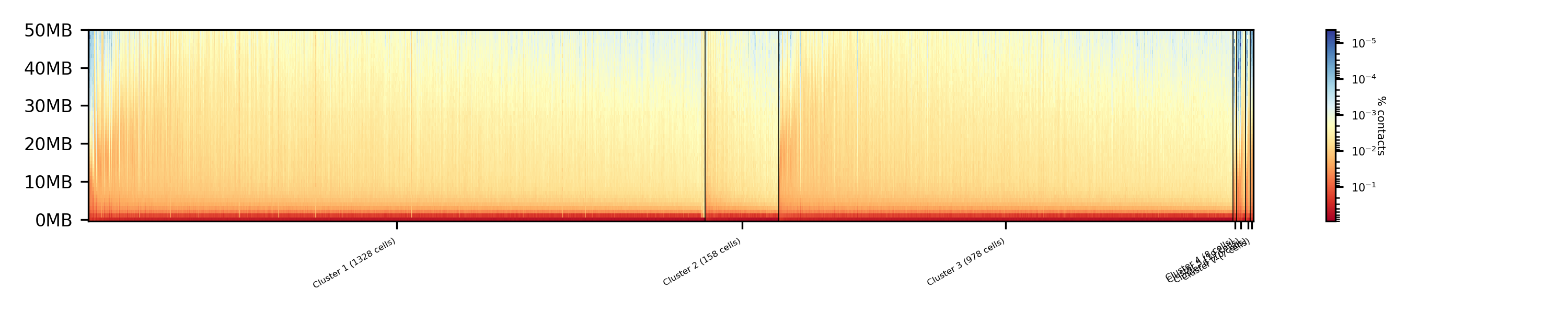
Clustering and dimension reduction based on A/B compartments will compute for each sample and each chromosome the A/B compartments, reducing the dimensions to the square root of the number of features i.e. in our example from 6.7 million to 2600.

$ scHicClusterCompartments -m nagano2017_corrected.scool --binarization --numberOfClusters 7 --clusterMethod kmeans -o clusters_compartments_kmeans.txt --threads 20

$ scHicClusterCompartments -m nagano2017_corrected.scool --binarization --numberOfClusters 7 --clusterMethod spectral -o clusters_compartments_spectral.txt --threads 20

To visualize the results run:

$ scHicPlotClusterProfiles -m nagano2017_corrected.scool --clusters clusters_compartments_kmeans.txt -o clusters_compartments_kmeans.png --dpi 300 --threads 20

$ scHicPlotClusterProfiles -m nagano2017_corrected.scool --clusters clusters_compartments_spectral.txt -o clusters_compartments_spectral.png --dpi 300 --threads 20

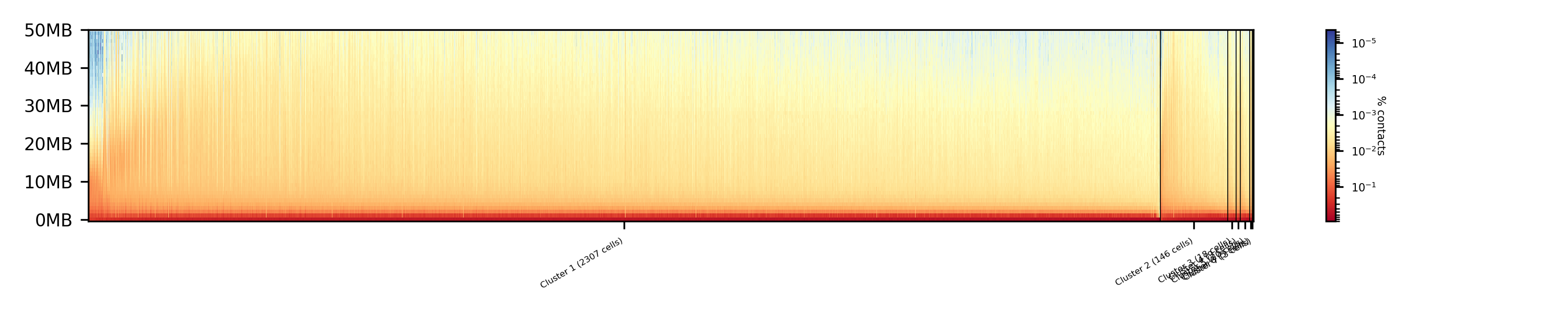
../_images/clusters_compartments_kmeans.png

../_images/clusters_compartments_spectral.png

The results of A/B compartment dimension reduction are mixed. The spectral clustering creates similar results as the non-dimension reduced clustering and is not useful. The kmeans clustering creates an equal distribution of the cells to the clusters,: but the profiles indicate the clustering itself is not good.

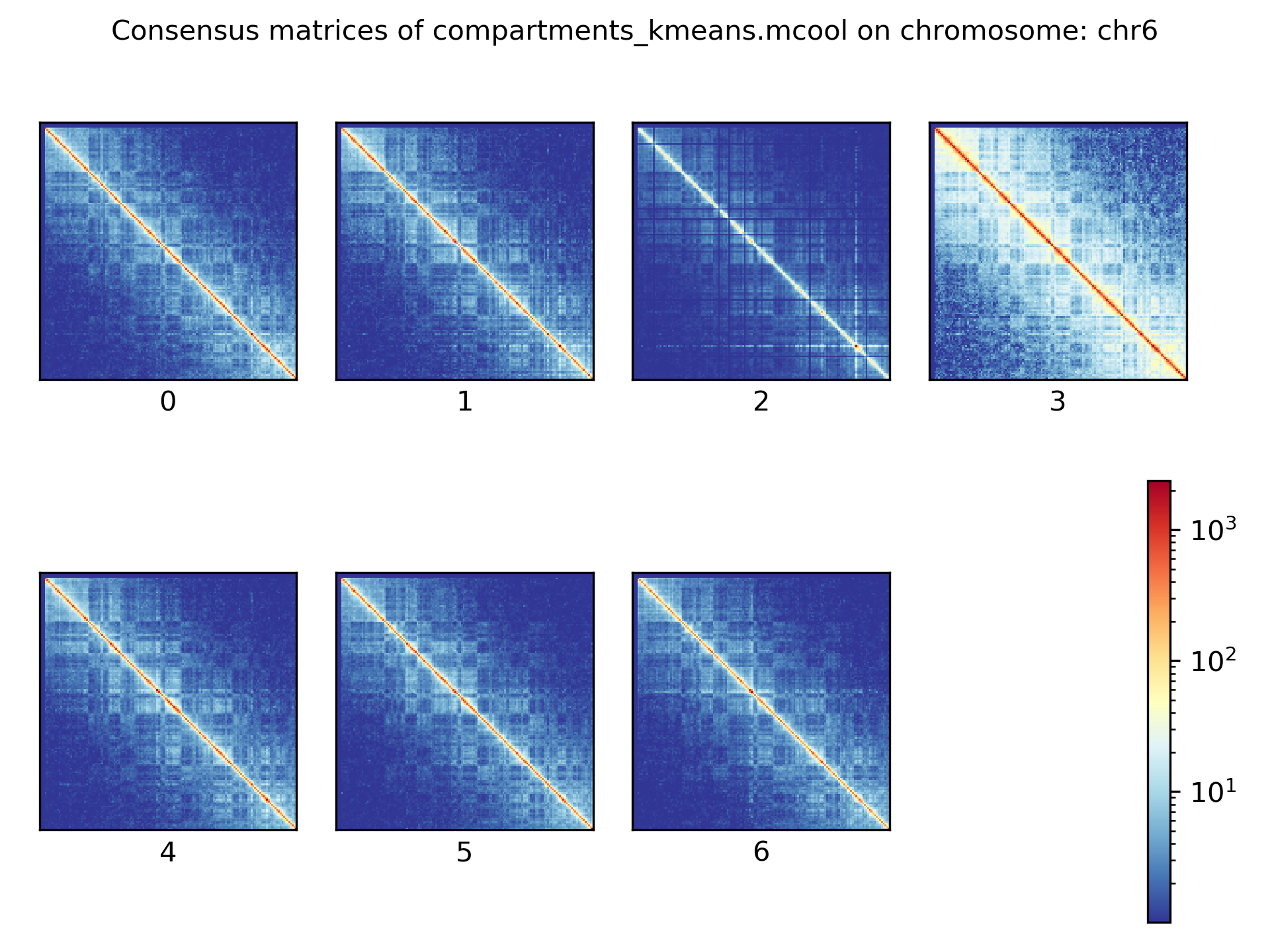
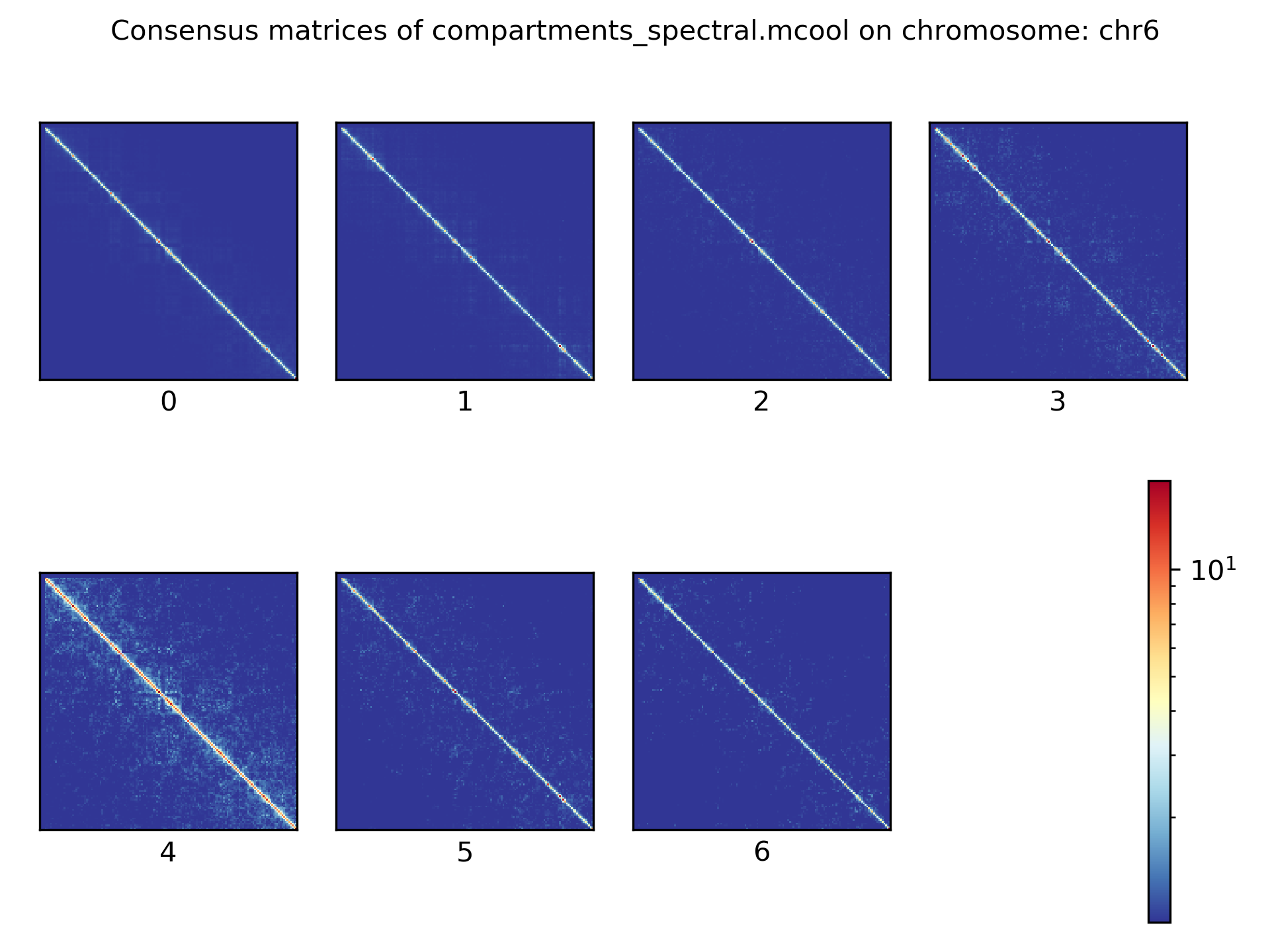
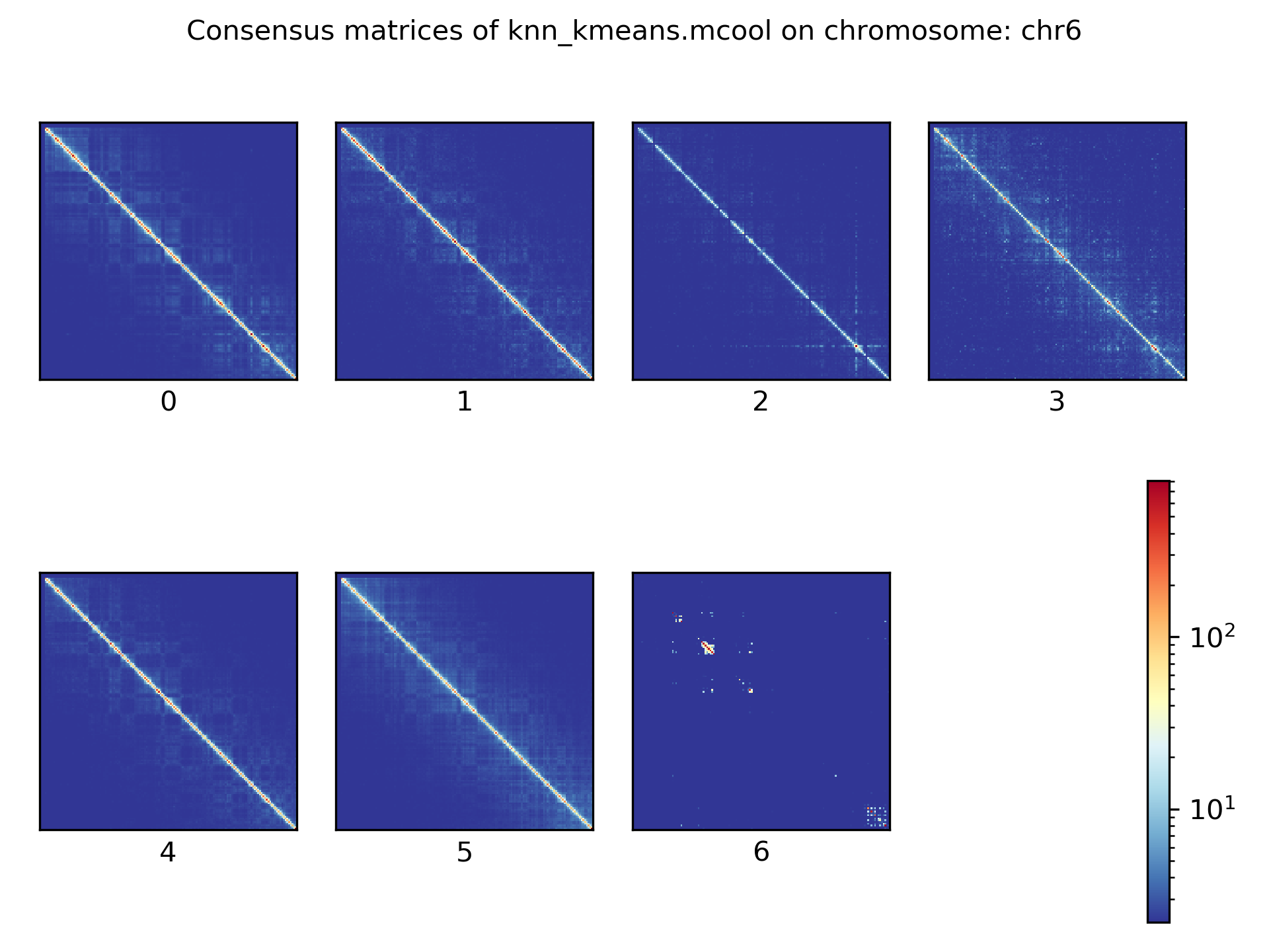
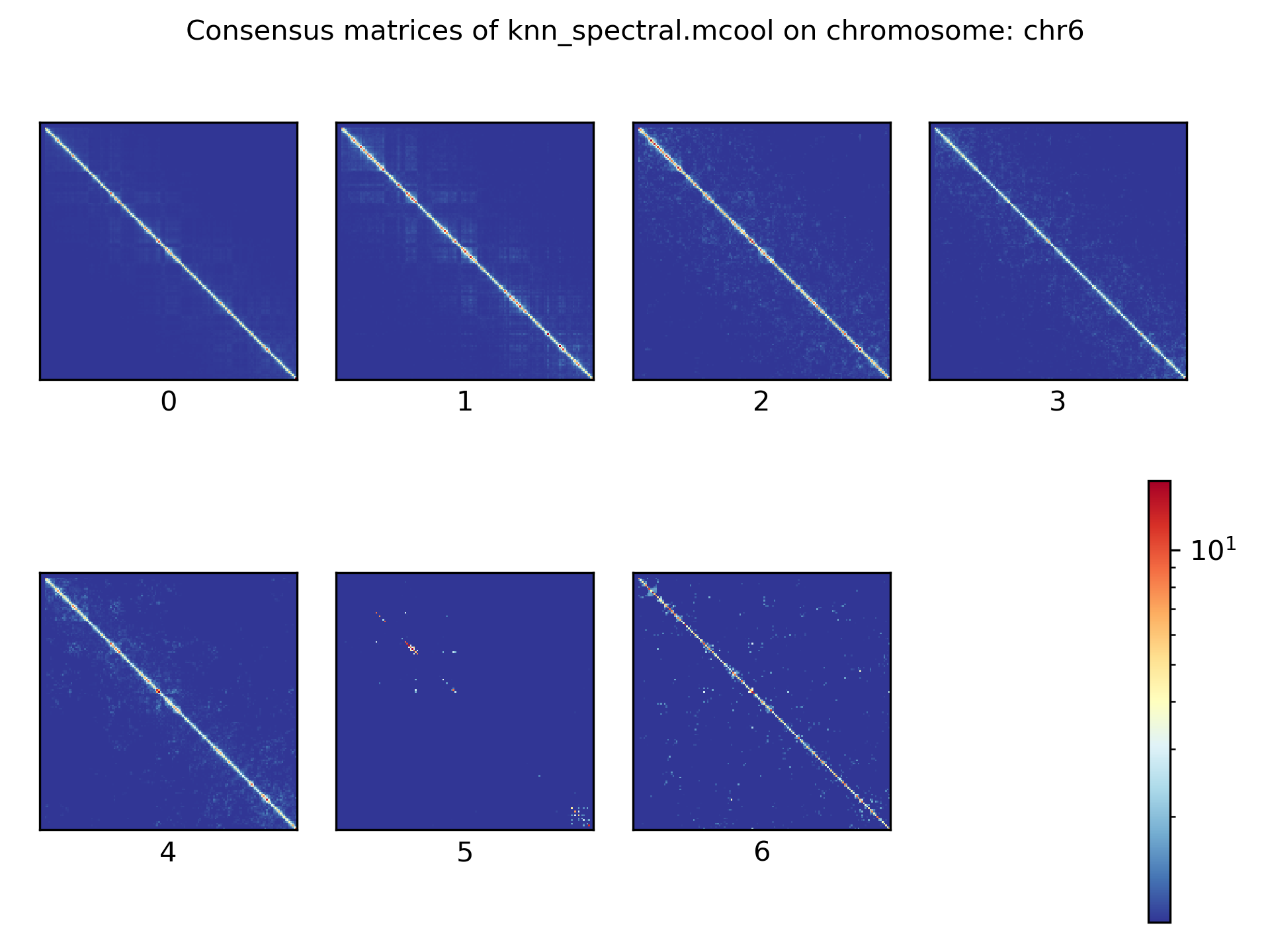
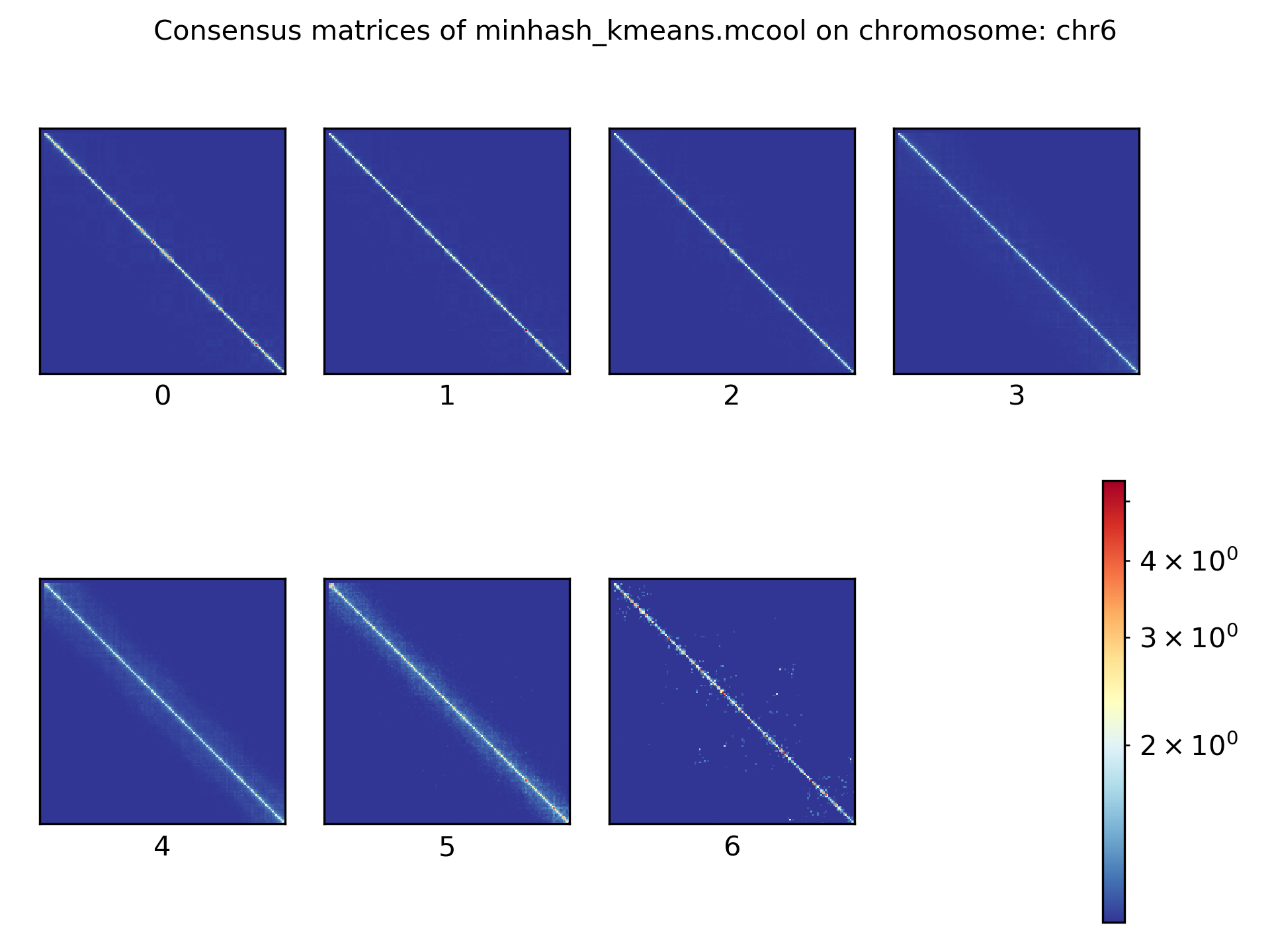
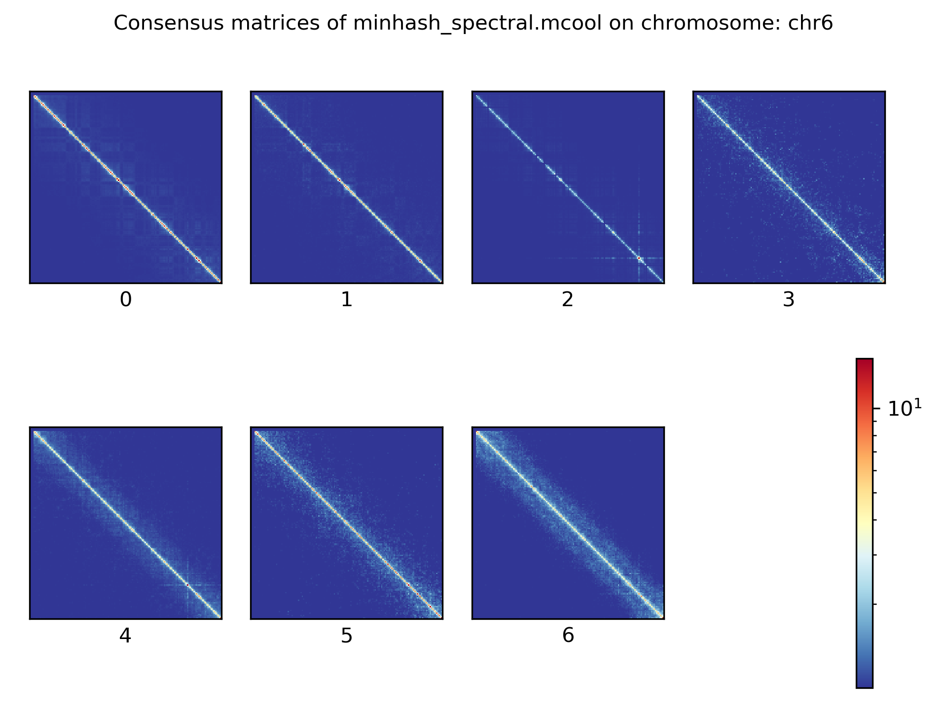
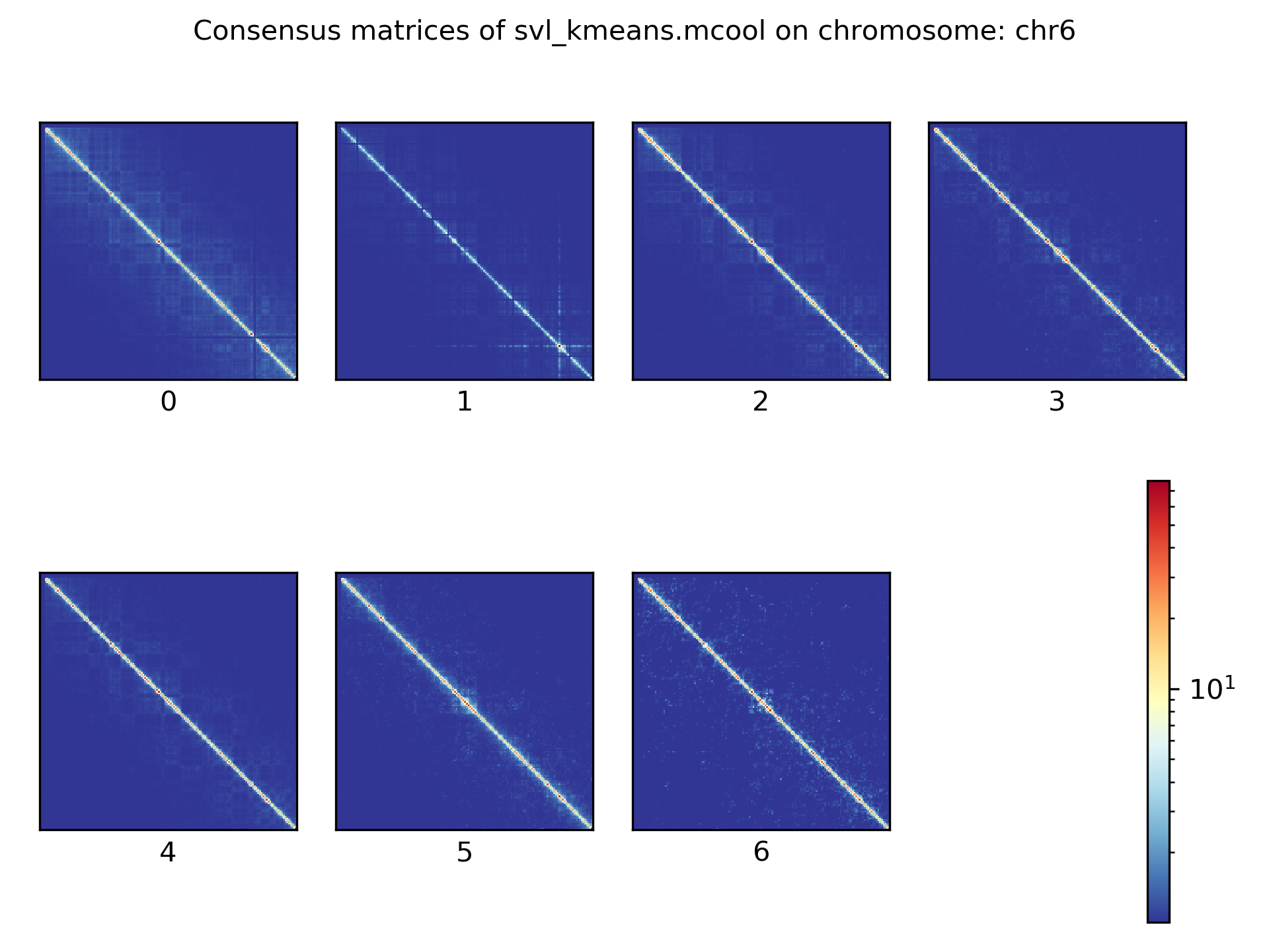
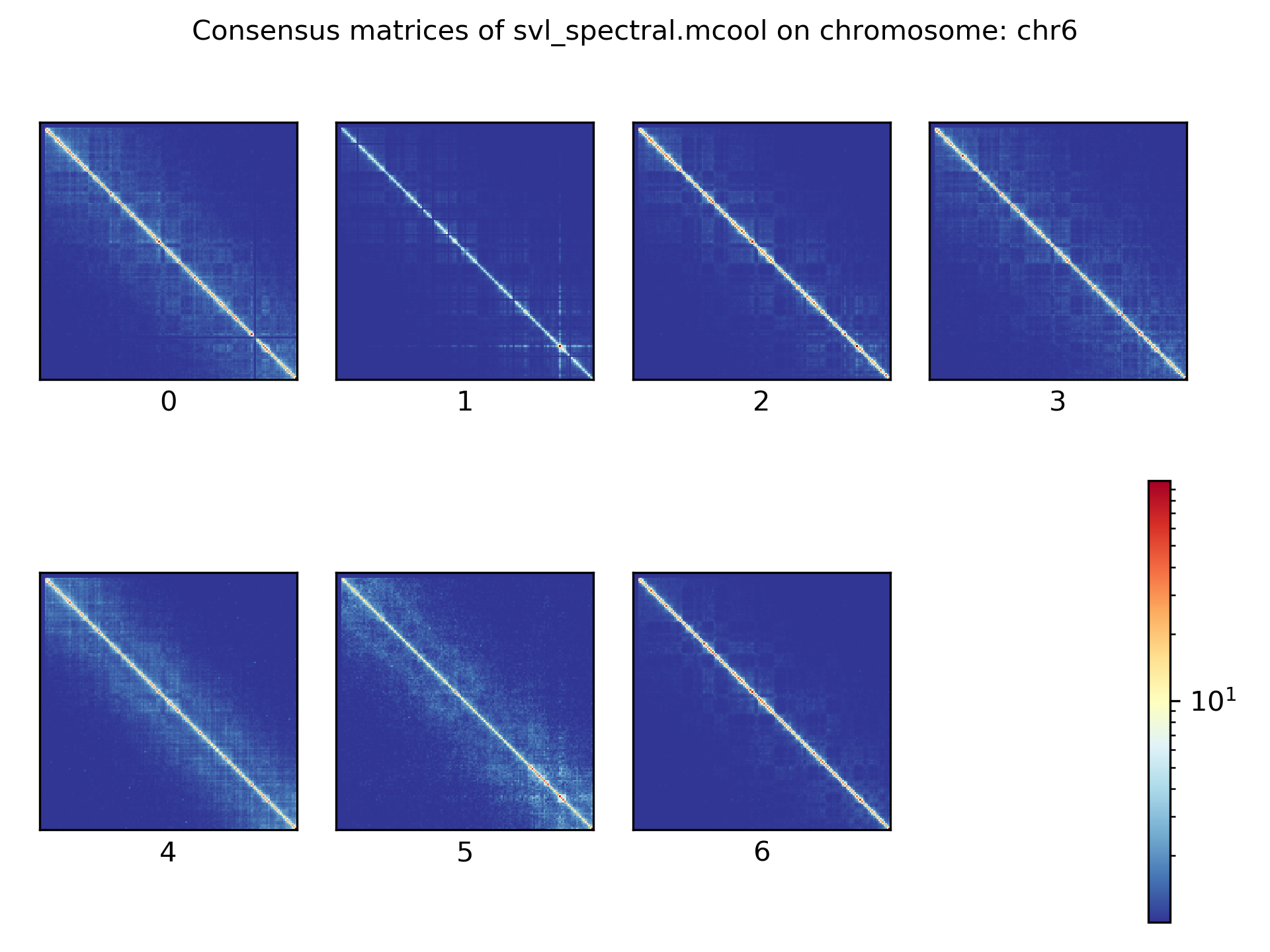
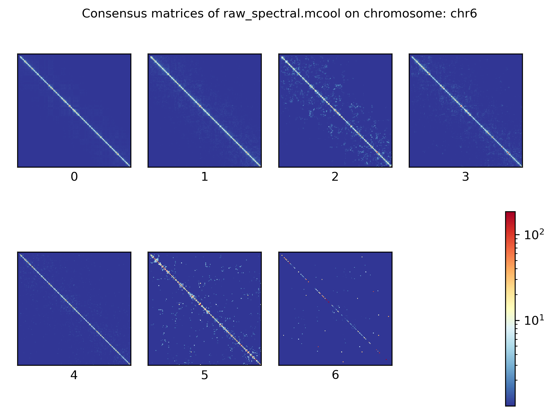
Consensus matrices ¶

The folding pattern of chromatin can be visualized by merging all Hi-C interaction matrices of one cluster together to one consensus matrix. First, the consensus matrices needs to be computed and in a second step be plotted.

$ scHicConsensusMatrices -m nagano2017_corrected.scool --clusters clusters_minhash_kmeans.txt -o consensus_matrix_minhash_kmeans.scool --threads 20

$ scHicPlotConsensusMatrices -m consensus_matrix_minhash_kmeans.scool -o consensus_matrix_minhash_kmeans.png --threads 20 --chromosomes chr6

In the following plots for different dimension reduction techniques are shown:

../_images/consensus_compartments_kmeans.png

../_images/consensus_compartments_spectral.png

../_images/consensus_minhash_spectral.png

Bulk matrix ¶

All single-cell matrices can be added together to one bulk matrix with the following command:

$ scHicCreateBulkMatrix -m nagano2017_corrected.scool -o nagano2017_bulk.cool -t 4

The resulting cool matrix can be plotted with HiCExplorer hicPlotMatrix:

$ hicPlotMatrix -m nagano_1MB_bulk.cool --log1p -o nagano_bulk.png --dpi 300 --chromosomeOrder chr1 chr2 chr3 chr4 chr5 chr6 chr7 chr8 chr9 chr10 chr11 chr12 chr13 chr14 chr15 chr16 chr17 chr18 chr19 chrX --fontsize 5 --rotationX 45

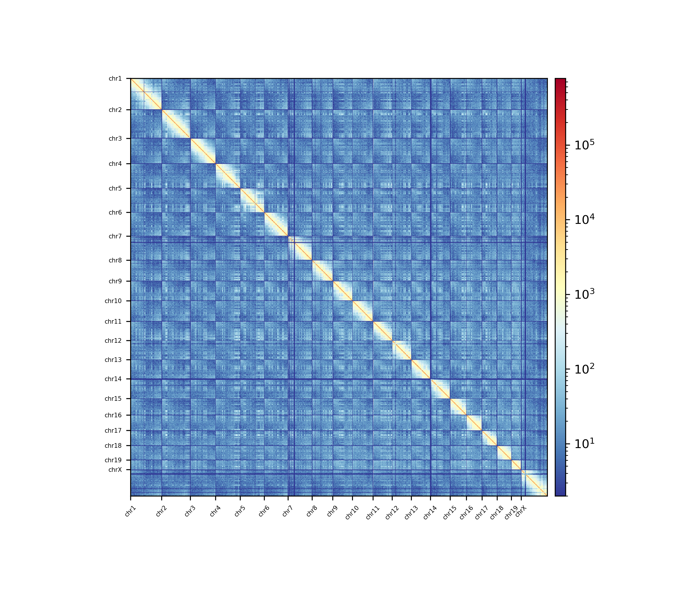
Nagano 2017 1 Mb resolution bulk matrix.